Income Consumption Curve Of A Perfect Complementary Commodities Is

Income Consumption Curve Wikipedia

Income Consumption Curve Wikiwand

Price Consumption Curve With Diagram Indifference Curve Economics

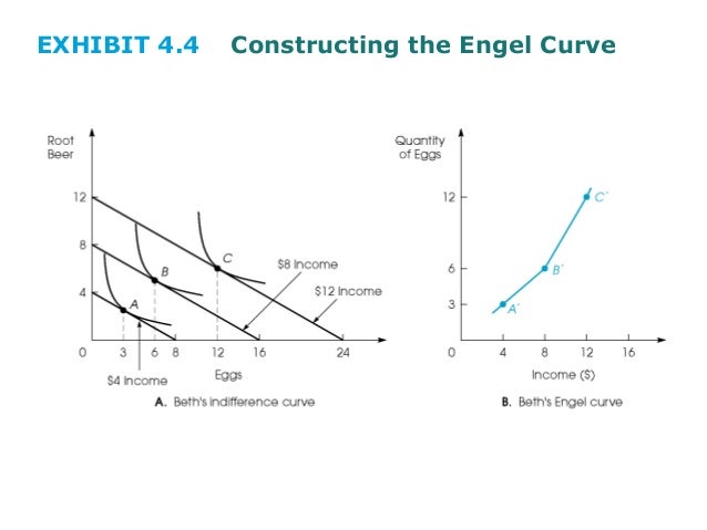
Notes On Income Consumption Curve And Engel Curve With Curve Diagram
Econ Income Consumption Curve Youtube
Price Consumption Curve Graph And Example
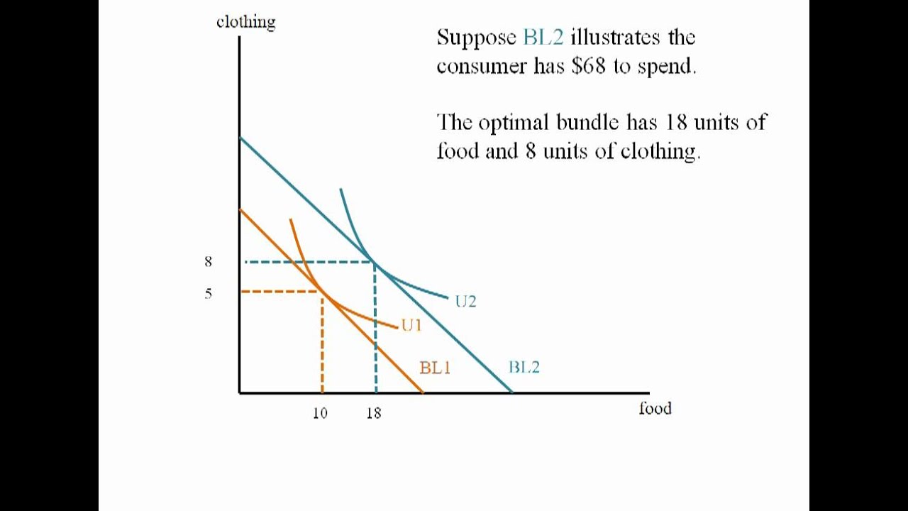
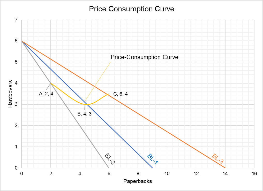
A as the price increases from p 0 to p 1 to p 2 to p 3 the budget constraint on the upper part of the diagram shifts to the left the utility maximizing choice changes from m 0 to m 1 to m 2 to m 3 as a result the quantity demanded of housing shifts from q 0 to q 1 to q 2 to q 3 ceteris paribus.
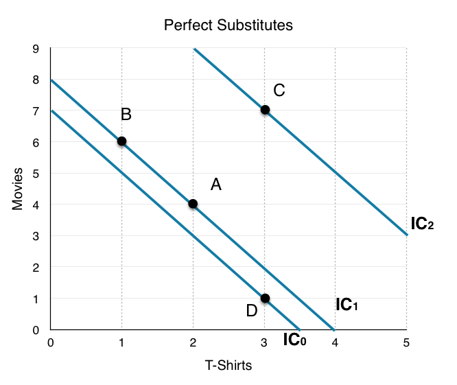
Income consumption curve of a perfect complementary commodities is. The theory of consumer choice is the branch of microeconomics that relates preferences to consumption expenditures and to consumer demand curves it analyzes how consumers maximize the desirability of their consumption as measured by their preferences subject to limitations on their expenditures by maximizing utility subject to a consumer budget constraint. Let us suppose x 1 and x 2 are perfect substitutes as shown in fig. Income consumption curve traces out the income effect on the quantity consumed of the goods. Upward sloping price consumption curve for x means that when the price of good x falls the quantity demanded of both goods x and y rises.
Two goods are perfect complementary goods an example of such goods would be gasoline and water in a car. As the level of consumption remains the same the income consumption curve for perfect complements is the diagonal line passing through the origin as shown in figure 5 on the left. If the price of any complementary. The following are the interesting case examples.
In case of perfect complements the same amount of goods will be consumed by the consumer irrespective of say income prices etc. D income consumption curve answer. Income effect for a good is said to be positive when with the increase in income of the consumer his consumption of the good also increases. 8 32 upward sloping price consumption curve is shown.
An example of housing. The rate gives a convex shape to the indifference curve. Indifference curves can be a straight line at a constant marginal rate of substiruuon b increasing marginal rate olsubstitutlon c increasing return to scale d none nf the above answer. Icc income consumption curve b lorenz curve c.
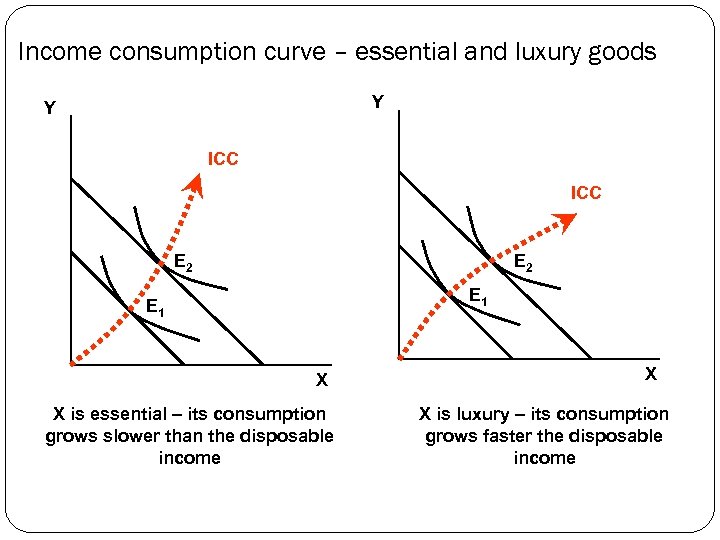
Income effect can either be positive or negative. Price consumption curve can have other shapes also. The simplest way to demonstrate the effects of income on overall consumer choice from the viewpoint of consumer theory is via an income consumption curve for a normal good see. This is the normal good case.
Two commodities are perfect substitutes for each other in this case the indifference curve is a straight line where mrs is constant. B the demand curve graphs. We obtain the upward sloping price consumption curve for good x when the demand for good is. When the income effect of both.
Under perfect competition the demand curve is a upward sloping b horizontal c downward sloping d vertical ans b 25. The basic premise behind this curve is that the varying income levels as illustrated by the green income line curving upwards will determine different quantities. The foundations of a demand curve. Single commodity consumption mode is a production possibility curve b law of equi marginal utility.
In this case the icc will coincide with the horizontal axes as shown in fig.

Consumer Reacts To Changes In The Price Of A Good Explained With Price Consumption Curve
Price Consumption Curve
Http Www2 Econ Iastate Edu Faculty Langinier Documents Pbset4 Answers Pdf
Mba 7003 1 1 Basic Conditions Demand

Income Effect Income Consumption Curve With Curve Diagram

Applications Of Indifference Curves Tutorsonnet
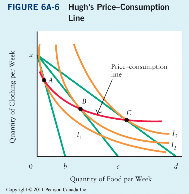
6 2 The Indifference Curve Principles Of Microeconomics

Income Offer Curve And Engel Curve Youtube

Normal Good Wikipedia
.svg)
Theory Of Consumer Choice Boundless Economics
Http Web Iitd Ac In Debasis Lectures Hul212 2017 Discussions Consumer Pdf
2 Consumer S Demand Analysis Structure O Factors

Notes On Convex Indifference Curves And Corner Equilibrium
